7.8 Thermal Analysis and Test

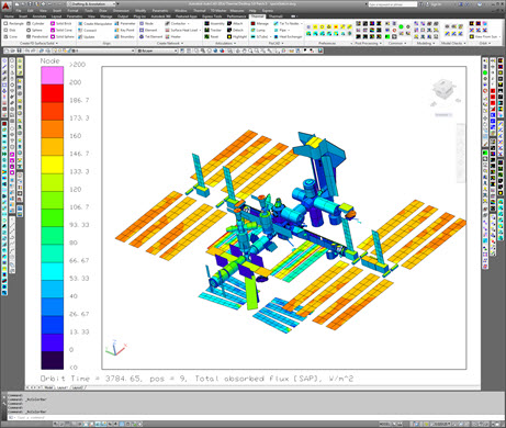
Finite Element Model and Analysis

Thermal system design strongly coupled with structures, orbit, and any component that generates heat or has strong thermal requirements. To create a thermal model, you will need:

• An orbital dynamics model or propagator, like STK
• An attitude dynamics model
• A satellite geometry, typically in the form of a CAD model, with proper material definitions
• Thermal modeling software, which usually accompanies a structural analysis model, like ANSYS or CAEplex
  • Boundary conditions

Just like the structural finite element model, the thermal finite element model creates a mesh of nodes that interact with neighboring nodes with first principles. Instead of passing strain and loads through the nodes, the thermal model passes heat through the nodes in the form of conduction, convection, and radiation. We’ll talk briefly about the maths underlying the thermal model for you to gain intuition as to thermal analysis results.

Space

“The finite element method creates a set of algebraic equations by using an equivalent governing integral form that is integrated over a mesh that approximates the volume and surface of the body of interest.  The mesh consists of elements connected to nodes.  In a thermal analysis, there will be one simultaneous equation for each node.  The unknown at each node is the temperature. Infinite element analysis, all surfaces default to perfect insulators unless you give a specified temperature, a known heat influx, a convection condition, or a radiation condition” [Akin].

“The temperature often depends only on geometry.  The heat flux, and the thermal reaction, always depend on the material thermal conductivity.  Therefore, it is always necessary to examine both the temperatures and heat flux to ensure a correct solution.  The heat flux is determined by the gradient (derivative) of the approximated temperatures.  Therefore, it is less accurate than the temperatures.  The user must make the mesh finer in regions where the heat flux vector is expected to rapidly change its value or direction.  The heat flux should be plotted both as to magnitude contours and as vectors” [Akin].

Spatially, the simple analytical conduction model that dictates the heat flowing from neighboring nodes in the x-direction is defined as:

Where i is the index of nodes. This equation can be iterated for the other two directions, y, and z. The heat going out of node i is analogous:

The heat that remains in the node is the difference between and . To find the temperature of this node over time indexed by , the physics are dictated by:

To handle radiation spatially, the surface nodes are subject to additional heat exchange defined by the Steffan Boltzmann equation. Note that the nodes on the surface are the only nodes to experience both conduction and radiation. The effect of radiation is passed on to neighboring nodes in a “trickle-down” effect. The numerical combination of conductive and radiative effects for finite element models is a field of active study [Vueghs et al.] and should be verified with a physical test as discussed in the next section.

Time

To propagate the node temperatures throughout time indexed by , we can use a time-marching solution:

Where the temperature difference d is

And is thermal diffusivity. To guarantee solution stability, the time step size is limited by the spatial difference and the thermal diffusivity through this relationship [Akin]:

Thermal Vacuum Testing

Testing in a thermal vacuum chamber is the closest we can get to simulating a space environment without actually testing in space. A thermal vacuum chamber simulates high vacuum and radiative/conductive heat transfer. High vacuum is achieved through specific pumps and may require staged pumping to transition from different categories of vacuum (rough > high).

Radiative heat transfer is achieved by covering the chamber’s inner surfaces with a black shroud, mimicking black body radiation. This shroud can be cooled to cryogenic temperatures to simulate the ambient temperature of space. Certain surfaces can be heated to or thermal lamps can be situated to simulate the radiation from the sun or other planetary bodies.

Under vacuum and subject to extreme heat conditions, the spacecraft and its embedded components will experience outgassing, thermal expansion, thermal cycling, and realistic heat transfer. Ideally, conditions are set such that the testbed shrouds, lamps, and conductive plates reflect the temporal and thermal profiles of the mission, which is affected by the orbit and ADCS. The spacecraft embedded electronics should be running as if the spacecraft were in space to replicate the internal power generated throughout a mission. The spacecraft should be littered with thermocouples and other temperature sensors at targeted points within the volume to verify that physical testing is similar to finite element results. The recorded temperatures during the test are then compared to the finite element model results to improve the predictive model’s accuracy/precision.

Artemis Thermal Profile

Suggested Activity