
The Chi-Square Distribution
Test for Homogeneity
OpenStaxCollege
[latexpage]
The goodness–of–fit test can be used to decide whether a population fits a given distribution, but it will not suffice to decide whether two populations follow the same unknown distribution. A different test, called the test for homogeneity, can be used to draw a conclusion about whether two populations have the same distribution. To calculate the test statistic for a test for homogeneity, follow the same procedure as with the test of independence.
The expected value for each cell needs to be at least five in order for you to use this test.
Hypotheses
H0: The distributions of the two populations are the same.
Ha: The distributions of the two populations are not the same.
Test StatisticUse a \({\chi }^{2}\) test statistic. It is computed in the same way as the test for independence.
Degrees of Freedom (df)df = number of columns – 1
RequirementsAll values in the table must be greater than or equal to five.
Common UsesComparing two populations. For example: men vs. women, before vs. after, east vs. west. The variable is categorical with more than two possible response values.
Do male and female college students have the same distribution of living arrangements? Use a level of significance of 0.05. Suppose that 250 randomly selected male college students and 300 randomly selected female college students were asked about their living arrangements: dormitory, apartment, with parents, other. The results are shown in [link]. Do male and female college students have the same distribution of living arrangements?
| Dormitory | Apartment | With Parents | Other | |
| Males | 72 | 84 | 49 | 45 |
| Females | 91 | 86 | 88 | 35 |
H0: The distribution of living arrangements for male college students is the same as the distribution of living arrangements for female college students.
Ha: The distribution of living arrangements for male college students is not the same as the distribution of living arrangements for female college students.
Degrees of Freedom (df):
df = number of columns – 1 = 4 – 1 = 3
Distribution for the test:\({\chi }_{3}^{2}\)
Calculate the test statistic: χ2 = 10.1287 (calculator or computer)
Probability statement: p-value = P(χ2 >10.1287) = 0.0175
MATRX
key and arrow over to
EDIT
. Press
1:[A]
. Press
2 ENTER 4 ENTER
. Enter the table values by row. Press
ENTER
after each. Press
2nd QUIT
. Press
STAT
and arrow over to
TESTS
. Arrow down to
C:χ2-TEST
. Press
ENTER
. You should see
Observed:[A] and Expected:[B]
. Arrow down to
Calculate
. Press
ENTER
. The test statistic is 10.1287 and the p-value = 0.0175. Do the procedure a second time but arrow down to
Draw
instead of
calculate
.
Compare α and the p-value: Since no α is given, assume α = 0.05. p-value = 0.0175. α > p-value.
Make a decision: Since α > p-value, reject H0. This means that the distributions are not the same.
Conclusion: At a 5% level of significance, from the data, there is sufficient evidence to conclude that the distributions of living arrangements for male and female college students are not the same.
Notice that the conclusion is only that the distributions are not the same. We cannot use the test for homogeneity to draw any conclusions about how they differ.
Do families and singles have the same distribution of cars? Use a level of significance of 0.05. Suppose that 100 randomly selected families and 200 randomly selected singles were asked what type of car they drove: sport, sedan, hatchback, truck, van/SUV. The results are shown in [link]. Do families and singles have the same distribution of cars? Test at a level of significance of 0.05.
| Sport | Sedan | Hatchback | Truck | Van/SUV | |
|---|---|---|---|---|---|
| Family | 5 | 15 | 35 | 17 | 28 |
| Single | 45 | 65 | 37 | 46 | 7 |
With a p-value of almost zero, we reject the null hypothesis. The data show that the distribution of cars is not the same for families and singles.
Both before and after a recent earthquake, surveys were conducted asking voters which of the three candidates they planned on voting for in the upcoming city council election. Has there been a change since the earthquake? Use a level of significance of 0.05. [link] shows the results of the survey. Has there been a change in the distribution of voter preferences since the earthquake?
| Perez | Chung | Stevens | |
| Before | 167 | 128 | 135 |
| After | 214 | 197 | 225 |
H0: The distribution of voter preferences was the same before and after the earthquake.
Ha: The distribution of voter preferences was not the same before and after the earthquake.
Degrees of Freedom (df):
df = number of columns – 1 = 3 – 1 = 2
Distribution for the test: \({\chi }_{2}^{2}\)
Calculate the test statistic: χ2 = 3.2603 (calculator or computer)
Probability statement: p-value=P(χ2 > 3.2603) = 0.1959
Press the MATRX key and arrow over to EDIT. Press 1:[A]. Press 2 ENTER 3 ENTER. Enter the table values by row. Press ENTER after each. Press 2nd QUIT. Press STAT and arrow over to TESTS. Arrow down to C:χ2-TEST. Press ENTER. You should see Observed:[A] and Expected:[B]. Arrow down to Calculate. Press ENTER. The test statistic is 3.2603 and the p-value = 0.1959. Do the procedure a second time but arrow down to Draw instead of calculate.
Compare α and the p-value:α = 0.05 and the p-value = 0.1959. α < p-value.
Make a decision: Since α < p-value, do not reject Ho.
Conclusion: At a 5% level of significance, from the data, there is insufficient evidence to conclude that the distribution of voter preferences was not the same before and after the earthquake.
Ivy League schools receive many applications, but only some can be accepted. At the schools listed in [link], two types of applications are accepted: regular and early decision.
| Application Type Accepted | Brown | Columbia | Cornell | Dartmouth | Penn | Yale |
|---|---|---|---|---|---|---|
| Regular | 2,115 | 1,792 | 5,306 | 1,734 | 2,685 | 1,245 |
| Early Decision | 577 | 627 | 1,228 | 444 | 1,195 | 761 |
We want to know if the number of regular applications accepted follows the same distribution as the number of early applications accepted. State the null and alternative hypotheses, the degrees of freedom and the test statistic, sketch the graph of the p-value, and draw a conclusion about the test of homogeneity.
H0 : The distribution of regular applications accepted is the same as the distribution of early applications accepted.
Ha : The distribution of regular applications accepted is not the same as the distribution of early applications accepted.
df = 5
χ2 test statistic = 430.06
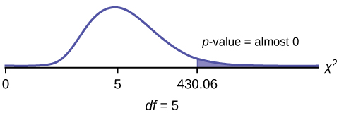
Press the MATRX key and arrow over to EDIT. Press 1:[A]. Press 3 ENTER 3 ENTER. Enter the table values by row. Press ENTER after each. Press 2nd QUIT. Press STAT and arrow over to TESTS. Arrow down toC:χ2-TEST. Press ENTER. You should see Observed:[A] and Expected:[B]. Arrow down to Calculate. Press ENTER. The test statistic is 430.06 and the p-value = 9.80E-91. Do the procedure a second time but arrow down to Draw instead of calculate.
References
Data from the Insurance Institute for Highway Safety, 2013. Available online at www.iihs.org/iihs/ratings (accessed May 24, 2013).
“Energy use (kg of oil equivalent per capita).” The World Bank, 2013. Available online at http://data.worldbank.org/indicator/EG.USE.PCAP.KG.OE/countries (accessed May 24, 2013).
“Parent and Family Involvement Survey of 2007 National Household Education Survey Program (NHES),” U.S. Department of Education, National Center for Education Statistics. Available online at http://nces.ed.gov/pubsearch/pubsinfo.asp?pubid=2009030 (accessed May 24, 2013).
“Parent and Family Involvement Survey of 2007 National Household Education Survey Program (NHES),” U.S. Department of Education, National Center for Education Statistics. Available online at http://nces.ed.gov/pubs2009/2009030_sup.pdf (accessed May 24, 2013).
Chapter Review
To assess whether two data sets are derived from the same distribution—which need not be known, you can apply the test for homogeneity that uses the chi-square distribution. The null hypothesis for this test states that the populations of the two data sets come from the same distribution. The test compares the observed values against the expected values if the two populations followed the same distribution. The test is right-tailed. Each observation or cell category must have an expected value of at least five.
Formula Review
\(\sum _{i\cdot j}\frac{{\left(O-E\right)}^{2}}{E}\) Homogeneity test statistic where: O = observed values
E = expected values
i = number of rows in data contingency table
j = number of columns in data contingency table
df = (i −1)(j −1) Degrees of freedom
A math teacher wants to see if two of her classes have the same distribution of test scores. What test should she use?
test for homogeneity
What are the null and alternative hypotheses for [link]?
A market researcher wants to see if two different stores have the same distribution of sales throughout the year. What type of test should he use?
test for homogeneity
A meteorologist wants to know if East and West Australia have the same distribution of storms. What type of test should she use?
What condition must be met to use the test for homogeneity?
All values in the table must be greater than or equal to five.
Use the following information to answer the next five exercises: Do private practice doctors and hospital doctors have the same distribution of working hours? Suppose that a sample of 100 private practice doctors and 150 hospital doctors are selected at random and asked about the number of hours a week they work. The results are shown in [link].
| 20–30 | 30–40 | 40–50 | 50–60 | |
|---|---|---|---|---|
| Private Practice | 16 | 40 | 38 | 6 |
| Hospital | 8 | 44 | 59 | 39 |
State the null and alternative hypotheses.
df = _______
3
What is the test statistic?
What is the p-value?
0.00005
What can you conclude at the 5% significance level?
Homework
For each word problem, use a solution sheet to solve the hypothesis test problem. Go to [link] for the chi-square solution sheet. Round expected frequency to two decimal places.
A psychologist is interested in testing whether there is a difference in the distribution of personality types for business majors and social science majors. The results of the study are shown in [link]. Conduct a test of homogeneity. Test at a 5% level of significance.
| Open | Conscientious | Extrovert | Agreeable | Neurotic | |
| Business | 41 | 52 | 46 | 61 | 58 |
| Social Science | 72 | 75 | 63 | 80 | 65 |
- H0: The distribution for personality types is the same for both majors
- Ha: The distribution for personality types is not the same for both majors
- df = 4
- chi-square with df = 4
- test statistic = 3.01
- p-value = 0.5568
- Check student’s solution.
-
- Alpha: 0.05
- Decision: Do not reject the null hypothesis.
- Reason for decision: p-value > alpha
- Conclusion: There is insufficient evidence to conclude that the distribution of personality types is different for business and social science majors.
Do men and women select different breakfasts? The breakfasts ordered by randomly selected men and women at a popular breakfast place is shown in [link]. Conduct a test for homogeneity at a 5% level of significance.
| French Toast | Pancakes | Waffles | Omelettes | |
| Men | 47 | 35 | 28 | 53 |
| Women | 65 | 59 | 55 | 60 |
A fisherman is interested in whether the distribution of fish caught in Green Valley Lake is the same as the distribution of fish caught in Echo Lake. Of the 191 randomly selected fish caught in Green Valley Lake, 105 were rainbow trout, 27 were other trout, 35 were bass, and 24 were catfish. Of the 293 randomly selected fish caught in Echo Lake, 115 were rainbow trout, 58 were other trout, 67 were bass, and 53 were catfish. Perform a test for homogeneity at a 5% level of significance.
- H0: The distribution for fish caught is the same in Green Valley Lake and in Echo Lake.
- Ha: The distribution for fish caught is not the same in Green Valley Lake and in Echo Lake.
- 3
- chi-square with df = 3
- 11.75
- p-value = 0.0083
- Check student’s solution.
-
- Alpha: 0.05
- Decision: Reject the null hypothesis.
- Reason for decision: p-value < alpha
- Conclusion: There is evidence to conclude that the distribution of fish caught is different in Green Valley Lake and in Echo Lake
In 2007, the United States had 1.5 million homeschooled students, according to the U.S. National Center for Education Statistics. In [link] you can see that parents decide to homeschool their children for different reasons, and some reasons are ranked by parents as more important than others. According to the survey results shown in the table, is the distribution of applicable reasons the same as the distribution of the most important reason? Provide your assessment at the 5% significance level. Did you expect the result you obtained?
| Reasons for Homeschooling | Applicable Reason (in thousands of respondents) | Most Important Reason (in thousands of respondents) | Row Total |
|---|---|---|---|
| Concern about the environment of other schools | 1,321 | 309 | 1,630 |
| Dissatisfaction with academic instruction at other schools | 1,096 | 258 | 1,354 |
| To provide religious or moral instruction | 1,257 | 540 | 1,797 |
| Child has special needs, other than physical or mental | 315 | 55 | 370 |
| Nontraditional approach to child’s education | 984 | 99 | 1,083 |
| Other reasons (e.g., finances, travel, family time, etc.) | 485 | 216 | 701 |
| Column Total | 5,458 | 1,477 | 6,935 |
When looking at energy consumption, we are often interested in detecting trends over time and how they correlate among different countries. The information in [link] shows the average energy use (in units of kg of oil equivalent per capita) in the USA and the joint European Union countries (EU) for the six-year period 2005 to 2010. Do the energy use values in these two areas come from the same distribution? Perform the analysis at the 5% significance level.
| Year | European Union | United States | Row Total |
|---|---|---|---|
| 2010 | 3,413 | 7,164 | 10,557 |
| 2009 | 3,302 | 7,057 | 10,359 |
| 2008 | 3,505 | 7,488 | 10,993 |
| 2007 | 3,537 | 7,758 | 11,295 |
| 2006 | 3,595 | 7,697 | 11,292 |
| 2005 | 3,613 | 7,847 | 11,460 |
| Column Total | 45,011 | 20,965 | 65,976 |
- H0: The distribution of average energy use in the USA is the same as in Europe between 2005 and 2010.
- Ha: The distribution of average energy use in the USA is not the same as in Europe between 2005 and 2010.
- df = 4
- chi-square with df = 4
- test statistic = 2.7434
- p-value = 0.7395
- Check student’s solution.
-
- Alpha: 0.05
- Decision: Do not reject the null hypothesis.
- Reason for decision: p-value > alpha
- Conclusion: At the 5% significance level, there is insufficient evidence to conclude that the average energy use values in the US and EU are not derived from different distributions for the period from 2005 to 2010.
The Insurance Institute for Highway Safety collects safety information about all types of cars every year, and publishes a report of Top Safety Picks among all cars, makes, and models. [link] presents the number of Top Safety Picks in six car categories for the two years 2009 and 2013. Analyze the table data to conclude whether the distribution of cars that earned the Top Safety Picks safety award has remained the same between 2009 and 2013. Derive your results at the 5% significance level.
| Year \ Car Type | Small | Mid-Size | Large | Small SUV | Mid-Size SUV | Large SUV | Row Total |
|---|---|---|---|---|---|---|---|
| 2009 | 12 | 22 | 10 | 10 | 27 | 6 | 87 |
| 2013 | 31 | 30 | 19 | 11 | 29 | 4 | 124 |
| Column Total | 43 | 52 | 29 | 21 | 56 | 10 | 211 |
